3.2.1. 17 Fractiles to be Estimated

There are 17 fractiles to be estimated: 6 threshold incomes, 6 average incomes, and 5 inter-fractiles. The following table describes what they correspond to.

Table 3.2. Definition and Notation of the 17 Fractiles to be Estimated

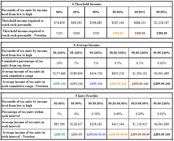
The threshold income labeled TI90 refers to the income level above which a tax unit belongs to the top decile and below which it does not. Six income thresholds were calculated: TI90, TI95, TI99, TI99.5, TI99.9, and TI99.99. ¹⁶ All of the income amounts are expressed in 2003 dollars, yet they do not take into account the cost of living differentials from one state to another.

The dollar amount in the AI90-100 category refers to the average income of the top decile. For instance, the richest 10 percent of Alabama’s tax payers earned about $137,646 on average in 2003 (current dollars). ¹⁷

This upper income class displays enough disparities to subdivide the top decile into 6 inter-fractiles: AI90-95, AI95-99, AI99-99.5, AI99.5-99.9, AI99.90-99.99, and AI99.99-100 ¹⁸ . Still considering the case of Alabama in 2003, the richest 0.01 percent earned about $10,128,674 that year. Such a high income could not be revealed by an income of $137,646 for the sole AI90-100 fractile.

The example of year 1940 gives reveals how sharp the differences can be from one state to another. For the households living in Arkansas that year, the threshold income TI90 is $9,354, while the threshold income of TI99.99 is $474,840. Meanwhile, $11,546,827 is the threshold of the richest 0.01 percent in Delaware. The same year, an income of about $47,000 makes a tax filer be part of the wealthiest 1 percent in Mississippi, but part of the wealthiest 10 percent in the District of Columbia.

In the whole sample (except Alaska), the District of Columbia has the highest TI90 threshold from 1917 to 1942, and again from 1944 to 1947, 1953-55, 1958, (except in 1918 with a third position after South Dakota and Nebraska, and in 1925 ranking second after Florida).

The year 2000 is an illustration of the peak in income levels reached by the top percentile that year. Among all the states, the highest income level of the AI99-99.5 fractile is recorded in Connecticut ($665,798). Still, that income level of the bottom half of the top percentile (AI99-99.5 in Connecticut) needs to be multiplied by more than 3.1 to reach the lowest values (among the states) of the highest fractile (AI99.99-100), which was recorded in West Virginia the same year ($665,798 * 3.1 < $2,096,212). Another example is that of the year 1982, when earnings of about $200,000 made a household belong to the AI99-99.5 fractile in Connecticut ¹⁹ but to the AI99.99-100 fractile in South Dakota ²⁰ .

Fractiles can be determined graphically using the cumulative curve. The cumulative distribution function plots the number of tax units (i.e. the number of households who filed a tax return) against the different income thresholds. For instance, the median interval simply corresponds to that bracket of income that contains 50% of the statistical population. However, to get a numerical estimation rather than a broad interval, income statisticians use the fact that typically, income cumulative curves fit the Pareto distribution fairly well at the upper tail.