4.3. Inter-State Inequality (ytop i,t / ybar US,t)
The estimation method applied at the state level is the same as Piketty and Saez’s at the national level. Therefore, the unweighted addition of top incomes across states (top panel) should match Piketty and Saez’s top income figures at the national level (bottom panel).
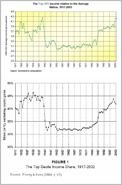
The reason why this calculation is done is to check the accuracy of the state estimates calculated here. Basic regressions of one against the other yield a (positive) R² of 0.8. The unexplained part of the correlation may be linked to several factors. One of them is that the two curves above are not identically defined. The former divides the top decile income by per household income (and typically exceeds unity) while the latter divides the top decile income by total income (and lies within unity). This should not affect the similarity in their respective trend, however. Another explanation refers to the unit income is measured with: Piketty and Saez constructed a tax-unit series to calculate income per tax unit, while we refer here to the income per household. Indeed, the availability of the data at the state level did not allow the state and national series to be identically constructed, despite all the adjustments already performed on the household series. 25
One may keep in mind that if the incomes of the top 10 percent do not exceed 4.5 times the national average during the entire time period, the top 0.01 percent reaches a peak of 380 times in 1916, and always lies above 150 times the national average, except for the 1940-1990 time interval.