5.2.1. β Convergence: Growth and Initial Income Level

Testing the Solow model of growth ²⁹ , the traditional regressions found in the empirical literature use a cross-country sample to perform a linear regression of growth rates on a constant term and the initial level of per-capita income. With i indexing U.S. states, the main equation is

(5.1)(1/T) . log [y _i,(t0+T)/y _i,t0] = α + β log [y _i,t0] + γX _i+ ε_it,

where:

T is the amplitude of the time-interval considered,

t ₀ is 1917 for the top decile, and 1913 for the top 1 percent,

log [y _i,(t0+T)/y _i,t0] is the overall growth rate of the BEA personal income per household in state i between year t ₀ and t ₀ +T,

(1/T) . log[y _i,(t0+T)/y _i,t0] is the annual growth rate of the BEA personal income per household in state i between year t ₀ and t ₀ +T,

y _i,t0 is the initial income level,

X _i represents one or more additional variables that may affect growth,

ε_i is a random error term, and

α, β, and γ are parameters to be estimated.

Initial income is entered in log form because that allows the coefficient β to be interpreted as the marginal effect of a one-percent increase in initial income on the growth rate. A negative value of β provides evidence supporting the convergence hypothesis of the Solow model. ³⁰

As Crain (2003) pointed it out, the definition of the growth rate (of income) is an issue. Whether the growth rate is defined one way or another, the estimated coefficients of an equation may change in sign. To illustrate his point, Crain opposed the ‘continuously compounded’ growth rate (as used in traditional convergence regressions) to the ‘least squares’ growth rate (that Crain derives from least squares trend regressions). In regressions based on the ‘least squares’ growth rates, the β coefficient is no longer statistically significant. Crain extended the analysis from income per capita to income per worker and concluded again on the sensitivity of the results to the growth rate definition, as shown in the table below.

Table 5.2. Barro-Type Test for State Income Convergence, 1969-1999

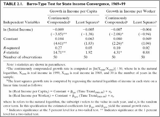
Source: Crain (2003, p. 28).

Taking this detail into account, the next figure distinguishes two definitions of growth rates, both being based on state average income per household. The first one is equal to the logarithm of the ratio of income level in year 2003 over the income level in year 1913: log(ybar ₂₀₀₃/ybar ₁₉₁₃). The second one is defined as the average of annual growth rates between 1913 and 2003. The results appear in panels (a) and (b) of the figure below, where each point represents a state.

Figure 5.3. Growth Rates versus Initial Income Level (a)

Figure 5.3. Growth Rates versus Initial Income Level (b)

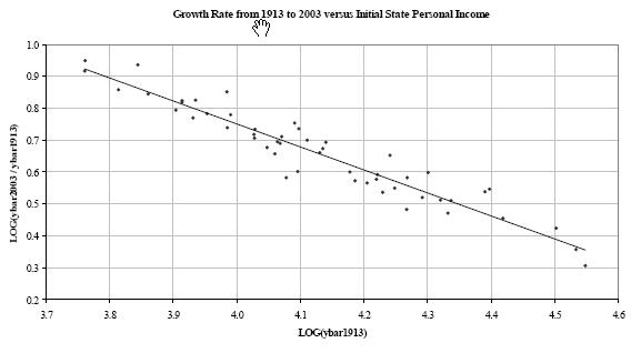
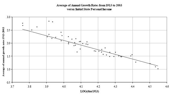
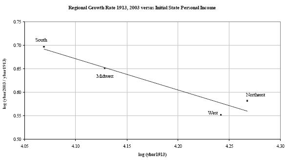
The declining trend clearly coincides with Barro and Sala-i-Martin’s results. To visualize where the states are located on the scatter plots, we aggregated the data at the regional level and what was expected clearly appeared in the figure below.

Figure 5.4. Regional Growth Rates versus Initial Income Level

As mentioned earlier, the data depicted in the two figures above are not derived from the IRS tables, but from the BEA state personal income data. The next section deals with the β convergence of the IRS incomes within the top 10 percent.