5.2.4. Spatial Auto-Correlation
The purpose of this section is to test the robustness of the previous results against the test of spatial-autocorrelation of the panel data set. A traditional measure of spatial auto-correlation is Moran’s I. It is used extensively in economic geography (Anselin, 1988, Janikas and Rey, 2005), and more and more by regional economists (Dall’erba and Le Gallo, 2005). Moran's I is a correlation coefficient (and therefore varies from negative one to positive one) weighted by the state-to-state distance matrix. More precisely, Moran’s I is defined as follows:
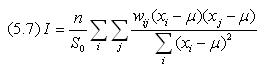
where n is the number of observations, w ij is the spatial weight matrix based on state-to-state distances, S 0 is the sum of all the elements of the spatial weight matrix, x i and x j stand for the error-term vector derived from the GMM regressions, μ is the arithmetic mean of x. Usually, the weight matrix takes the inverse of the distance between state i and j, so that a high value of Moran’s I indicates a cluster effect and a low value the independence of nearby points. “The Moran's I value that indicates spatial independence of values (or the lack of spatial autocorrelation) is a negative number close to zero” (Hare, 2001). We exacerbate here the differences in state-to-state distances by raising their values to power (minus) two:
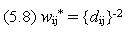
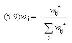
where {d} represents the distance between regions i and j. It is also common in the spatial data literature to normalize the rows of the weight matrix so that each row sums to unity, and so that S 0 equals n in the formula defining Moran’s I. 33
Applied to the present data set, Moran’s I takes the value of -0.2341, which tends to justify the fact that the attractive forces of economic poles spread locally, but not globally. In other words, polarization is a self-reinforcing phenomenon that pulls further apart high and low-income areas: high-income states exert attraction on neighboring areas (and these peripheral areas bring more income revenues to the core) but not to the extent of reaching rural remote areas where poverty falls into the trap of hysteresis, where low-income states stayed with low-income levels simply because it was the case in the previous time period.