5.3.2. Incomes of Top 90-95 and 95-99 Percent Record Increasing Dispersion
The incomes of the 90-95 and 95-99 percent revealed an increase in dispersion across states over time. This result contrasts with the previous section where average income and income of top 1 percent both recorded a sharp decrease in dispersion across states over time (except after the mid 1980s). This opposition is suggested twice: once with the coefficient of variation regressed on time (table below), and another time with graphs of the standard deviation (figure below). 34
| Dependent variable: CVt(ytop i,t) | AI 90-95% | AI 95-99% | Top 1% |
| Time coefficients | 1,167.4 * | 1,550.6* | -0.0047 * |
| * Statistically significant at the 1% confidence level. | |||
The figure below displays income dispersion within the top decile, measured by the coefficient of variation, and the decomposition of its ratio (standard deviations and means are expressed in 2003 dollars).
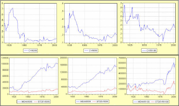
A common point to all three groups is that the increasing portion of the CV curve after the mid-1980s is accounted for by a rise in both the mean and the standard deviation. However, the differences among them lie on the opposition mentioned earlier: Considering the coefficient of variation of the two fractiles of the 90-99 percent interval, one may notice their respective decrease between the mid-1930s and the late 1970s. This downward trend occurred along with a sharp increase in their mean income, but with a slow and smooth rise in their standard deviation. As for the top percentile CV, it experiences a drop between 1939 and 1980 due to opposite trends in the standard deviation (decreasing) and the mean (increasing), the same way the dispersion of average income did (bottom panel of Figure 5.6).