6.2.1. The Functional Form of the Lorenz Curve

The Lorenz curve literature suggests different functional forms of the Lorenz curve: exponential function, power function, log-normal function, etc., all involving the estimation of a certain number of parameters. Among all these parametric forms, which one is relevant here? None is fully satisfactory, but the one chosen here fits the Pareto distribution of income, as assumed and used earlier with the estimations of fractiles within the top decile. Applying the Pareto distribution to the functional form of the Lorenz curve is an old and followed tradition in the empirical literature. ³⁷ Moreover, the Pareto functional form of the Lorenz curve limits to one the number of parameters to be estimated. Multiplying the number of parameters in the model specification, however appealing it can be, raises complications in terms of interpretation of the results and the computation of the estimates.

With x being the cumulative proportion of the household population, and y being the cumulative percentage of income earned, the parametric function of the Lorenz curve is supposed to be of the form:

(6.2)

How best to represent the Pareto form of the Lorenz curve? The probability density function associated with the Pareto distribution is the same as the probability density function (PDF) associated with the Pareto interpolation technique described in Chapter 3:

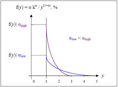
With y standing for income, α a scalar, and k, the minimum level of income in the distribution, f(y) = α kα/ y(1+α), the Pareto PDF, captures well the 80-20 percent rule. f(y), the “probability” or fraction of the population that earns a small amount of income per person (y), is rather high for low-income levels, then decreases steadily as income y increases: The higher the values of α, the wider the gap of inequality.

The parameter α corresponds to the coefficient calculated earlier in the estimation of fractiles of the upper decile, based on the Pareto interpolation method. There is one α coefficient attributed to each income bracket displayed in the Statistics of Income tables annually and at the state level.

In the case of France in the time-period 1900-1910, Piketty ³⁸ used a Pareto coefficient of 2.6, which means an α coefficient of 1.625 as α = b / (b – 1). In the case of our panel data on the United States, the α coefficients calculated in Chapter 3 average at 2.1 for all states and years, and display a very low standard deviation (0.57), as expected. ³⁹