6.3.2. Inequality Regressions on Gini Coefficients

As earlier, we use GMM estimation to assess the correlation link between inequality and economic growth. Like Chapter 5, economic growth is measured by the growth rate of state average income per household. Unlike in Chapter 5, the inequality indicator is no longer a fractile but the Gini matrix. The regressions lead, once again, to a negative correlation between the two variables. ⁴⁰

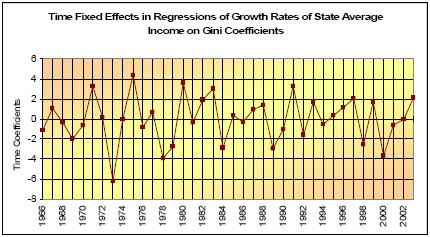
However, the introduction of time fixed effects in the inequality equation leads to regression coefficients that display neither consistency in sign, nor strong significance, as shown in the figure below.

Figure 6.5. Time Fixed Effects in Growth Regressions with Gini Coefficients

An alternative way of examining the whole distribution is to consider ‘opposite’ percentiles, such as P10 vs. P90, P25 vs. P75, take their percentage share in total income as displayed on the Lorenz curve (L10, L90, and L25, and L75), and calculate their respective ratios. ⁴¹ More details are available in the next section.